As the solar industry matures, financiers and developers are increasingly asking for P90 analyses before investing in a solar project. This is no longer solely a utility-scale practice, as commercial projects are increasingly being financed based on P90 estimates.
Yet many developers have not thought deeply about P90 analysis, especially those who focus on C&I projects rather than utility-scale. And while developers can simply take a 3 to 4% haircut to the project value and move on, there are opportunities to gain (or lose) 1 to 2% of project value if you know which questions to ask. We’ll dig into those here with a deep-dive into P90 adjustment math.
The baseline
First, a very brief primer on P90 adjustments:
What is a P90 adjustment?
A downward adjustment to the estimated output you assign to a solar array, to account for year-to-year variability in the system’s performance.
Why would we do it?
If a solar array is financed, especially with debt, then you want to make sure that you have enough cash flow (or bill offset) each year to cover the payments. Simply taking the “average” historical weather has the downside that you should expect to underperform half of the time—sometimes by a lot.
How do you do it?
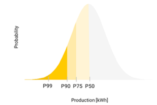
P90 values are obtained by simulating a system’s production over multiple years, determining how much variability there is from year to year, primarily driven by the weather (measured by the standard deviation) and then calculating the haircut necessary to outperform the estimated value 90% of the time. For a normal distribution, the 90% confidence value is exactly 1.28-times the standard deviation.
For further reading, we recommend these good primers from Heatspring and NREL.
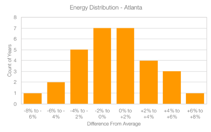
We’ll start by digging deep into one location: Atlanta. Over 30 years, the average annual energy production for Atlanta is 1,506 kWh/kWp, with a standard deviation of 47 kWh/kWp, which is about 3.1% of the mean value. In other words, about 68% of the annual results will happen within +/- 3.1% of the average sunlight. With a standard deviation of just over 3%, this means that the P90 haircut is about a 4% deviation from the average. In this case, the P90 production value would be 96% of 1,506 kWh/kWp, or 1,446 kWh/kWp.
When we plot the results in a histogram, we can see that the results are pretty close to a normal distribution: most of the results are closest to the average, with a few years that are further away from the average.
Multi-location
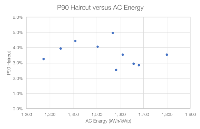
Next, let’s look at how this P90 analysis looks for a number of different cities across the United States. What is striking is that across a range of locations where the annual sunlight varies by nearly 50%, the P90 haircut is pretty consistent from one location to the next. It ranges from 2.5% for the most consistent location to 4.9% for the one with the greatest variation, with eight of the ten values in a narrow range from 2.8% to 4.4%.
It may seem counterintuitive, but there is no clear correlation between sunlight and variability. Sunnier locations are not inherently more variable than cloudier places—or vice versa.
Symmetry and skewness
All of the above analysis assumes a normal distribution in sunlight. However, is that true? A normal distribution assumes that the distribution is balanced: that the left tail is equal in number and magnitude to the right tail. But we can hypothesize that it may be more common to have a bad year (caused by excessive clouds or storms) than an equally good year. After all, there aren’t many events that will amplify the sun!
Statistically, we can measure this by calculating the “skewness” (asymmetry) of a distribution. A negative skewness indicates that the distribution has a larger negative tail, whereas a positive skewness shows a larger positive tail. A perfectly normal distribution will have a skewness of zero.
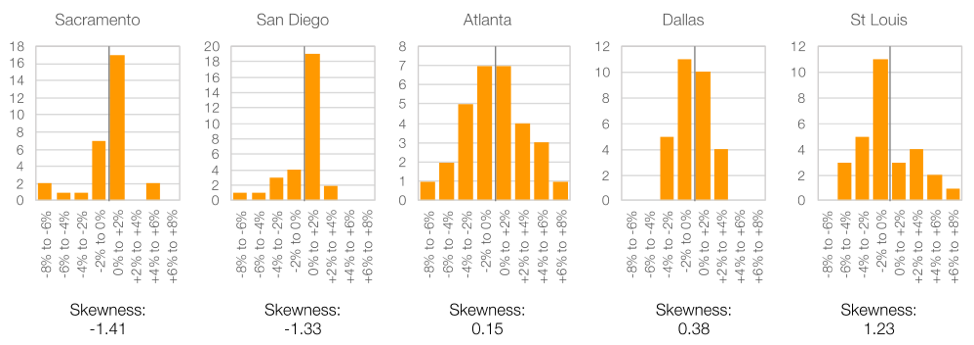
Across our ten locations, we can see there is actually a wide range of skewness values: six values are negative, but four are positive. Across all of them, the average is -0.30.
If we look at a few of the distributions in detail, we can see that there are clearly visibly differences between a dataset with a negative skew vs. a dataset with a positive skew.
Impact of skewness on P90
We can show the importance of skewness by re-calculating the P90 value bottoms-up: rather than assuming a normal distribution and calculating the P90 value from the standard deviation, we can alternatively sort the 30 values, and take the mid-point between the 27th and 28th value—in other words, the value at which 27 of the 30 years of production (90%) are greater.
In this “manual” approach, we can see that for most of the heavily skewed distributions, the bottoms-up approach will change the P90 haircut by 0.5% or more—dropping the value for the negatively-skewed distributions, or raising it for the positively-skewed distributions. Not a huge difference, but a fairly material sum when considered that this can be a “free” source of value in one direction or the other simply by running an extra analysis.
Weather source (Prospector vs TMY2)
We can also see if the weather source changes the overall variability. All of the analysis above was done using the TMY2 data set (https://rredc.nrel.gov/solar/old_data/nsrdb/1961-1990/tmy2/). This is a ground-based source with 30 years of data, from 1961 to 1990. We can run a similar analysis on Solar Prospector, which is a satellite-based source with 12 years of data, from 1998 to 2009.
Across our ten locations, the overall average P90 haircut is strikingly similar between TMY2 and Prospector: 3.6% for TMY2, and 3.4% for Prospector. Yet at any one location, the differences can be quite large: for four of the ten locations, there is more than a 1% difference between the TMY2 result and the Prospector result. Once again, just by asking which weather source is used, you may be able to change the value of the system by a full percent or more.
Monthly vs. annual variability
Probably the most striking result of the analysis is how much greater the variability is on a monthly basis. If we were to isolate a single month and compare 30 years of data, the variability is much larger. Recall that the average standard deviation for the annual values is 2.8%—the average standard deviation in monthly values is 10.2%. So, the resulting P90 haircut would be correspondingly higher: 13.1% for monthly values compared to 2.6% for annual values.
Another way to think about it: on an annual basis, the average change in production from one year to the next is 2.5% (up or down). But on a monthly basis, the average change from year to year is 11.1%.
What we’re seeing here is essentially the flip-side of the ‘law of large numbers.’ When adding up performance over a full year, a bad winter can be offset by a good summer, and vice versa. If you keep collecting enough data, things tend to revert to the mean. But if you isolate a smaller period of time (say, a month), then you will see much greater variability.
Luckily, projects aren’t financed based on their monthly P90 values. However, this is a lesson that we shouldn’t jump to conclusions about a project’s overall health based on the performance in one single month. These changes could very well be caused by the weather and may be 10% better (or worse) the following year.
One final point: all of the analysis above is backward-looking. We unfortunately don’t have detailed data for future weather. But given the reality of climate change and the corresponding impact on weather, it is reasonable to expect that the variability of weather in the future will actually increase, even if the averages remain the same. There is a good discussion of uncertainty (and its impact on P90 calculations) by Solargis here.
As the solar industry matures, we should all expect P90 performance adjustments to become more common, not less so. And while a 3 to 4% adjustment is perfectly fine for the budgetary step, developers should absolutely look deeper before locking in the final production value. Changing the weather source, or adjusting for the skewness of the underlying data, can push the project value 1% or more in either direction. All it takes is a bit more analysis.


Tell Us What You Think!