
When someone says, “My simulation results aren’t lining up with what I used to see in PV Watts,” our first troubleshooting step (and the most common source of problems) is the weather file. While everyone thinks about the choice of modules or inverters as a major driver of the energy yield, those aren’t as important as the weather file, which can swing yield by 5 to 10%. Yet many engineers barely think about weather files until very late in the solar design process.
Weather files are too important to not understand. Here we will explain the different types of weather files, how they are constructed and why financiers will ask for a discount vs. the standard weather file outputs.
Know your source: satellite vs. ground-based sources
There are two major types of weather files: satellite-based and ground-based. Ground-based files are more ubiquitous in the United States: “TMY2” and “TMY3” files are based on physical weather stations that measure the sunlight (aka irradiance) and temperature over the course of multiple years.
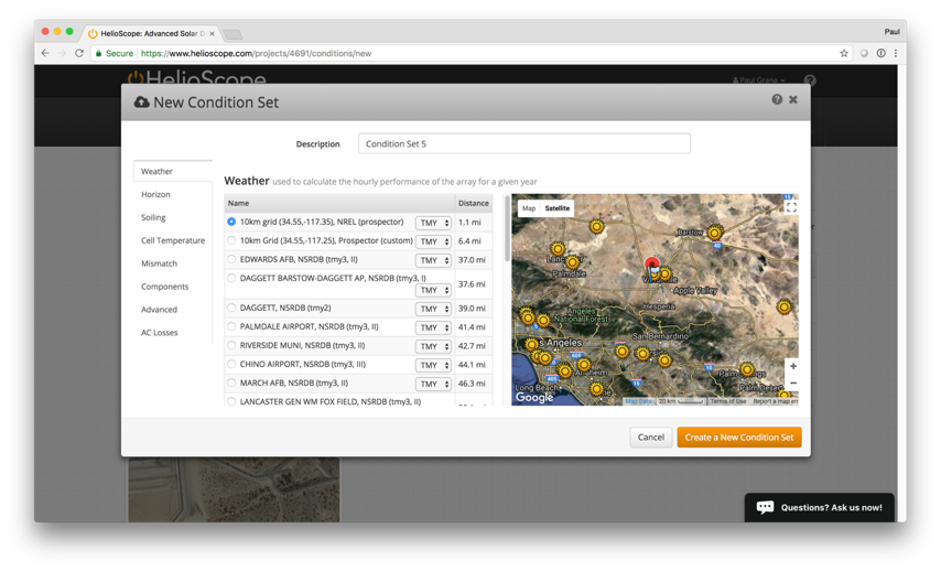
Figure 1: Weather file selection in HelioScope
Satellite-based weather files such as NREL’s Solar Prospector are based on satellite images, where the image is used to calculate the amount of cloud-cover over each spot on the planet. Then a methodology calculates the irradiance loss based on the cloud cover.
In PVWatts, only TMY2/TMY3 files are available, so many people who use PVWatts are baselined to ground-based weather files. There are also premium weather files (of both types) from firms such as Clean Power Research, Solargis, AWS Truepower and 3TIER.
Outside the U.S., satellite-based weather is more common. It is pulled from sources such as Meteonorm and PVGIS, though there are also a number of ground-based sources such as EnergyPlus and SolarGis.
The two types of weather sources can actually have fairly significant differences. As seen from the chart below, Prospector weather files are often more aggressive than TMY3, with an average difference of +2.9% greater production across 20 U.S. metro areas (and some sites seeing nearly a 10% difference):
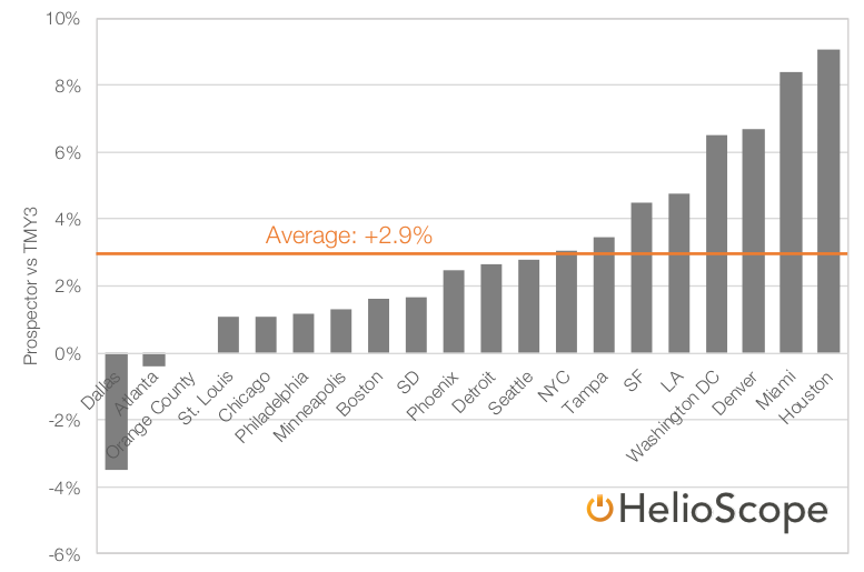
Figure 2: Prospector weather results vs. TMY3 for Top 20 U.S. metro areas
How TMY is constructed
TMY files are constructed to provide a realistic view of what a “typical” year looks like at a location. There are two objectives in making sure that the data is typical:
- Ensure that the overall simulation averages are in line with historical averages
- Ensure that the day-to-day and hour-to-hour variations preserve the “noisiness” of the real-world
Note that an “average year” (say, taking the 20-year average for each hour) would satisfy the first objective (having results that are in line with averages), but would not satisfy the second objective. Specifically, all of the highest and lowest values would be smoothed out.
Instead, we construct a “typical year”: calculate the average irradiance and temperature across all of the January months, and then select the single year where the January is closest to the average. But once that “typical January” is selected, all of the specific hourly results are maintained. The result is a synthetic year where the values of each month come from a different year, but the overall sunlight is very close to average, with a normal amount of very sunny/very cloudy days.

Figure 3: Illustrative construction of typical year
This is also why the hourly simulation results from performance models sometimes look funny. The January values might be from 1998, while the February values might be from 2003:

Figure 4: Example hourly simulation file using typical year data
Choosing a weather file
There isn’t a right or wrong source for weather, though there are different approaches for how developers think about weather files.
Some will decide that they prefer to use a specific type (either satellite-based or ground-based), and only use that. The primary argument for satellite-based weather is the consistent methodology: the cloud calculation approach is applied uniformly across regions. For a developer comparing projects across different states or counties, they can be confident that the differences between sites are not caused by differences in how the weather stations are maintained. On the other hand, while ground-based weather sources can vary based on the physical maintenance, they are generally considered to be higher quality, since they are directly measuring the same conditions that the prospective solar array will see.
Others will take a hybrid approach: switching between ground-based and satellite-based on proximity—or even running multiple simulations and using the average (or minimum) value.
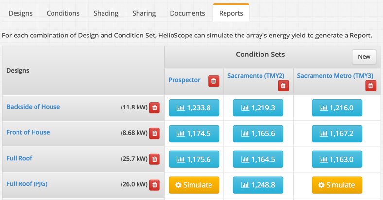
Figure 5: Report summary with multiple weather sources
Annual variability and P50 vs. P90
The world is an uncertain place. Even if we had perfect information about what had happened in the past, there are significant differences from year to year. Often, the production of an array can vary by as much as 5 to 10% from year to year.
If we were to look at multiple years of weather data, the overall amount of sunlight follows a normal distribution (a bell curve):
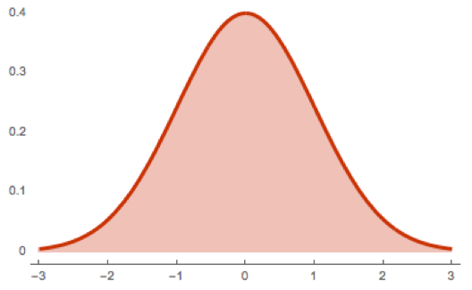
Figure 6: Example normal distribution
In light of that distribution of sunlight, solar developers will talk in terms of “PXX” for finding a spot on the distribution. Specifically, a P50 value is the spot on the curve where half of the years should be greater than the value—in other words, the middle of the curve and the average value. Then, P90 is the spot on the curve where you expect to outperform the value 90% of the time.
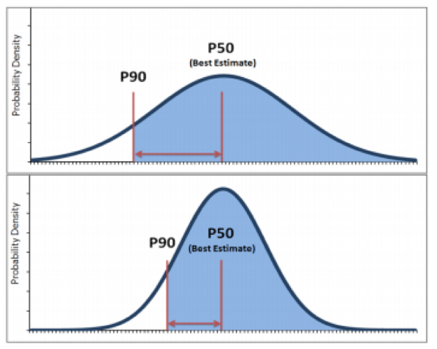
Figure 7: P50 and P90 adjustment (Credit: AWS Truepower)
The average, or P50, is the right approach when you are trying to get the most neutral understanding of what a system will do. Since a solar array is essentially a series of cash flows, then arguably the fairest calculation is to base the value off of the average production over that time period.
However, someone is often depending on the revenue from that array, either to pay down a loan used to finance the array or for investment income. And keep in mind that an array will underperform its “average” value 50% of the time (and will also over-perform half of the time). This is why financiers will often require that an array is financed based on the P90 production rather than P50.
While a P90 calculation sounds complicated, it is not that difficult to generate:
- First find a dataset with multiple years. In the U.S., this includes TMY2 and Solar Prospector.
- Calculate multiple years of production. Here, more is better—ideally you would want to run every year available (XX years for Prospector and 30 years for TMY2).
- “Standardize” the multiple years into a normal distribution. For those interested, there is a function in Excel that can do this, =standardize(), or alternatively we have a template calculator here.
- Finally, using the normal distribution, find the point on the curve that corresponds to the place where 90% of the distribution is to the right. Again, our online calculator does this automatically. Note that if you were going to run a different level, say P80 or P95, you would just calculate a different point on the curve.
In practice, a P90 production value will typically be 2 to 4% lower than the corresponding TMY/P50 value. While it isn’t fun to lose 2 to 4% of the project value in financing, this will ensure that the production is less likely to underperform expectations (though it will still underperform 10% of the time).


Tell Us What You Think!